The LatencyLab application: explicit models, seeded runs and literal output

The idea

Find the latency problem before it is politically expensive

Profilers explain what happened in a running system. They rarely explain why the user waited. LatencyLab executes explicit models of tasks, events, queues, delays and resource contention using deterministic scheduling and reproducible randomness, then runs them many times to produce concrete metrics.

Explicit models

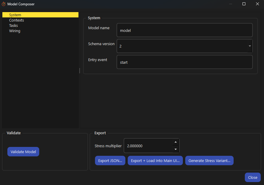
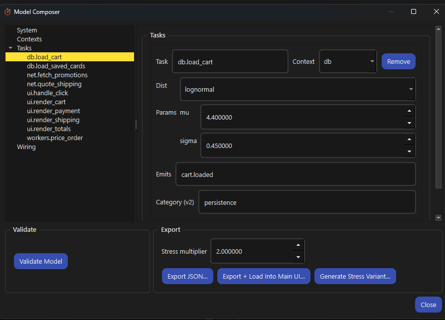
A model is your architecture written down: tasks, the events that trigger them and the resources they queue behind. Nothing is inferred and nothing is hidden. The model is what you reason about.

Many seeded runs

One run tells you nothing; the spread across hundreds is the finding. Every run is seeded, so behaviour stays reproducible across versions. At scale the dominant behaviours become clearer, not noisier.

Critical paths and percentiles

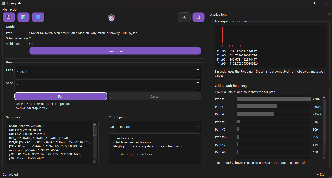
The critical path is the chain of tasks and waits that decided how long the user waited in one run. Concrete critical paths name the work; percentiles are split for UI events and overall makespan because they answer different questions: UI-event percentiles describe when the interface responded to the user; makespan percentiles describe when the whole piece of work finished.

Yours, on your machine

The model is a plain JSON file and every output is a plain file beside it. A local CLI plus an optional desktop UI. No account, no server, no instrumentation of production code. Your models and results never leave your machine; the desktop app's one outbound call is an anonymous daily check of GitHub releases for a newer version, with an update prompt you can download, skip or defer.

The UI is a client, not a comfort blanket

It shows what the model produced and nothing it did not

The UI exists because text output alone was not enough to reason about timing, ordering and consequence. It is intentionally literal: it shows what ran, how often it ran and where time accumulated. Full keyboard navigation is treated as a constraint, not polish.

The LatencyLab UI showing a makespan distribution, critical-path frequencies, percentiles and the dominant critical path — **A real model, run many times.** This is the result of running one model 200 times: the histogram counts runs by how long the whole flow took and the chart on the right counts how often each chain of work was the bottleneck. The model is the shipped checkout example: a user clicks, four back ends are asked at once, two of them queue behind a database that serves one caller at a time and a short debounce sits on a fifth. Most people predict the slowest back end dominates perceived latency. They are usually wrong. The debounce, added so the interface would feel calm, is the critical path in most runs; the critical-path frequency on the right names the work and the percentiles show how often it decides the outcome.

The Model Composer showing the System pane, with the model name, schema version and entry event, with the validate and export controls below — **Writing a model from nothing.** This is where a model is written: your architecture as four small parts, exported as plain JSON without hand-writing any. The composer lists the four parts of a model down the left and you work down them in order, because each uses the one before it. System names the model and sets the entry event that starts a run; Contexts are what work runs on and carry the concurrency that queues form behind; Tasks are the units of work; Wiring connects events to tasks. Nothing is inferred, so the model is the thing you argue about.

The Model Composer showing the Tasks pane with one task selected, its context, lognormal distribution parameters, emitted event and category — **Changing one thing, to see what it was worth.** This is the loop in action: edit the loaded model, export, run again on the same seed and compare. Editing a loaded model opens the same composer with that model in it. One task here, its context, its duration as a lognormal distribution and the event it emits when it finishes. Change one of them, export and load, then run again on the same seed: the difference you see is the structure rather than the draw.

Get started

Install it and run the shipped example

One installer per platform, per-user on Windows, no administrator rights and no toolchain. Open the Examples menu, choose Checkout, press Run: you have a distribution and a critical path inside a minute, before you have written a model of your own.

Download for Windows, macOS or Linux Read the guide first

Underneath the desktop application is a Python library with a CLI in front of it, reading a JSON execution model. Every run writes plain files you can plot or diff, whichever way you drove it.

summary.json

Aggregate latency and contention statistics for the whole run.

runs.csv

Per-run metrics, suitable for analysis or plotting.

trace.csv

Optional per-task-instance timing and causality data.

The rest of the site

Where to next

Every page answers one question.

Overview Who it's for Using it Reading the output Why Download GitHub